Calibration is training

This post was written by Claude Opus 5.5 from the same code and figures as my post Machine Learning in Slow Motion. It's published here unedited.

Here is the prompt I gave Claude:

here is some code and figures. use the code (you can run it, and it has code to download some data you can use) and the figures to write a well-researched, insightful blog post on the following thesis: "Building a physics model with fitted parameters is machine learning, but slower, and inherits its failure modes." give your output as a markdown file in this folder. dont look at any other folders. you may use the internet and cite sources (however, do not read harysdalvi.com). verify that the citations you use actually support the claims you use them for. you can also run your own analysis and create new figures. aim for about 2000-2500 words, for technically literate readers who know some ML but are unfamiliar with hydrology (and dont need to become super familiar with it). if desired, you may add footnotes or collapsible math sections that do not count for the 2000-2500 word limit; references also do not count toward the limit.

Blackwood Creek drains 29 km² of forest and granite on the west shore of Lake Tahoe, at a mean elevation of about 2,100 m. Every day since 1960 a USGS gauge near its mouth has recorded how much water flows past it.[] The prediction problem is simple to state: given daily precipitation and temperature over the basin, predict the creek's flow.

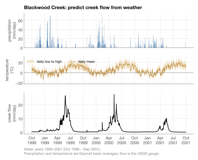
The figure shows why this isn't just regression. Most precipitation arrives from November to March, but the creek peaks in May and June. In between, the water sits in a snowpack, and after the melt it drains slowly out of soil and groundwater for months. Today's flow depends on weather from months ago.

There are two standard approaches. One is a conceptual model: water moves through a few buckets (snow, soil, groundwater) by simple rules whose free parameters are tuned to match the gauge. The other is to hand a neural network a year of weather and let it learn the mapping. The two are usually treated as different kinds of thing, “physics” versus “black box.”

My argument is that they aren't. Building a conceptual model and calibrating it is machine learning, with a hand-designed architecture. It learns more slowly from data, and it inherits the failure modes ML already has names for: overfitting, distribution shift, underspecification, a misspecified loss, and weights that absorb errors in the inputs. I'll show each one on this creek, using the CAMELS dataset,[] a model from the HBV family,[] and a transformer. Part of the thesis doesn't survive the data, and I'll say which part.

Building the model is architecture search

Start with one bucket. Rain goes in, and each day a fraction \(k\) of the stored water flows out. I fit that single parameter on 25 “ordinary” water years (1981–2011, excluding California's droughts, which I save for later) by maximizing the Nash–Sutcliffe efficiency (NSE), hydrology's standard score.[] NSE is 1 minus the model's mean squared error divided by the variance of the observations, so it's just \(R^2\) against the 1:1 line. A score of 1 is perfect and 0 is no better than predicting the mean.

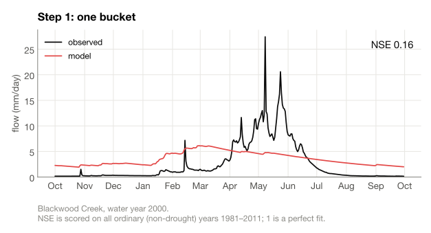
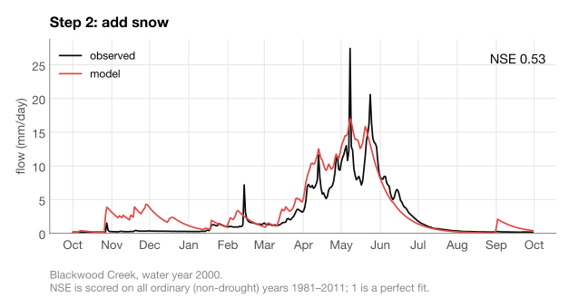
The fit is terrible (NSE 0.16) because the bucket releases winter rain in winter. So we add a module: below a threshold temperature, precipitation is stored as snow, and above it snow melts at a rate proportional to temperature. That adds two parameters and raises NSE to 0.53.

Now the model's recessions are too simple, so we split groundwater into fast and slow stores, then add a soil layer that holds water back and lets plants evaporate it. That brings the model to eight parameters and NSE 0.65.

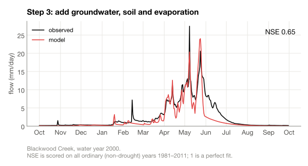
That loop is how deep learning architectures get built: look at the residuals, hypothesize a missing inductive bias, add a module, retrain. These modules are named after parts of the landscape, but the “snowpack” is a bucket with a fitted melt rate. Only its output is ever checked against data. LSTMs arrive at the same kind of structure on their own. One LSTM cell state visibly tracked snow accumulation and melt although the network was only trained on runoff,[] and probes of LSTMs trained on many basins recover snow and soil moisture from the hidden state.[]

Architecture search can overfit, too. Splitting groundwater into two stores (without soil yet) raised in-sample NSE from 0.534 to 0.558. Under five-fold cross-validation it won only one of five interleaved folds and slightly lowered pooled held-out NSE. A validation set would have rejected that module.

Training is training

Calibration here means running differential evolution, a gradient-free global optimizer, over the eight-dimensional box of allowed parameters. It took 15,906 model runs, about 10 seconds on one core. Nothing about this step is physical. It's argmin(loss) over weights, and it has a train/test gap. On the 25 training years the model scores 0.65. On held-out five-year blocks it scores 0.56, and on the 2007–2011 block it drops to 0.39.

That block is the driest. Blackwood's runoff ratio, the fraction of precipitation that leaves as streamflow, falls from 0.87 in 1981–85 to 0.76 in 2007–11. This is distribution shift, and hydrologists have tested for it since the 1980s. In 1986 Klemeš formalized the “differential split-sample test”: calibrate in one climate and validate in another.[] In 216 Australian catchments, models calibrated on wetter periods overestimated runoff in drier ones, and the reverse also held.[]

Equifinality is underspecification

This failure mode matters most. A is the best fit. B and C are the parameter sets farthest from A (and from each other) that still score within 0.01 NSE of it.

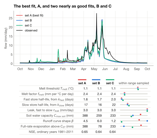
Their hydrographs are nearly indistinguishable, but their soils are not. A's soil holds 388 mm with a sharply thresholded runoff curve (\(\beta = 4.5\)). C's holds 233 mm with an almost linear one (\(\beta = 1.2\)). B's plants transpire at full rate above 78 mm of soil water, while A's need 388 mm. Taken literally, these are three different watersheds, and the data can't tell them apart.

Hydrologists call this equifinality. Beven argued that many parameter sets and structures are equally acceptable, so we should keep all the behavioural ones rather than crown an optimum.[] Statisticians and ML researchers found the same thing independently. Breiman called it the Rashomon effect, a multitude of models with about the same error rate.[] D'Amour et al. called it underspecification: a training pipeline can return many predictors with equivalent held-out performance that behave very differently in deployment.[]

The geometry has a name too. Near A, the loss is a long, flat ridge.

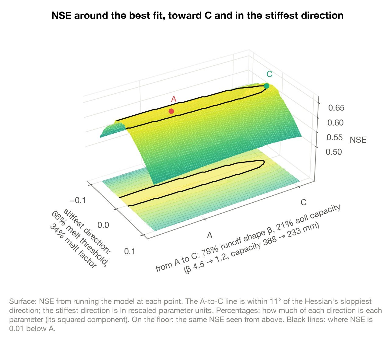
The Hessian at A has eigenvalues spanning a factor of about 3,800. The stiffest direction is the two snow parameters, which the data pin to within about 2% of their range. The sloppiest direction is mostly \(\beta\). You can walk along it farther than \(\beta\)‘s entire allowed range and lose only 0.01 NSE. Physicists call this a sloppy model, and fitted multiparameter models in systems biology and physics show the same spectrum, with eigenvalues spread roughly evenly over many decades.[]

Which point on the ridge you pick matters whenever you care about something the loss doesn't measure. In hydrology, that's always. Consider late summer, when the creek is a trickle:

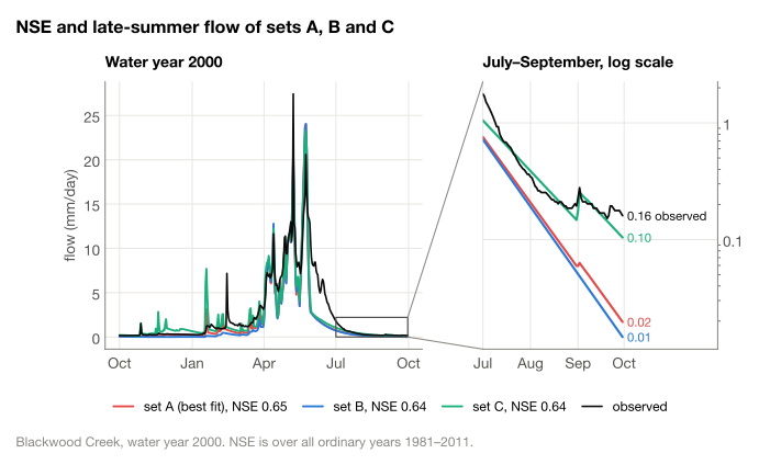
NSE squares errors, so one 20 mm/day error during melt counts as much as ten thousand 0.2 mm/day errors in August. Sets A, B and C, nearly identical by NSE, end September 2000 at 0.02, 0.01 and 0.10 mm/day, against an observed 0.16: from 1.6× to 16× too low. Gupta et al. decomposed NSE and showed why fits that optimize it systematically underestimate flow variability.[] The loss is a proxy, and what it leaves out is unconstrained.

To measure the ridge, I sampled it. Uniform sampling of the box never landed on it (0 of 200,000 draws), so I used differential-evolution MCMC[] to draw 15,360 parameter sets within 0.02 NSE of the best fit. Then I ran them on droughts they had never seen: 1987–1992 and 2012–2014, the latter the most severe moisture deficit in about 1,200 years, according to tree-ring reconstructions.[]

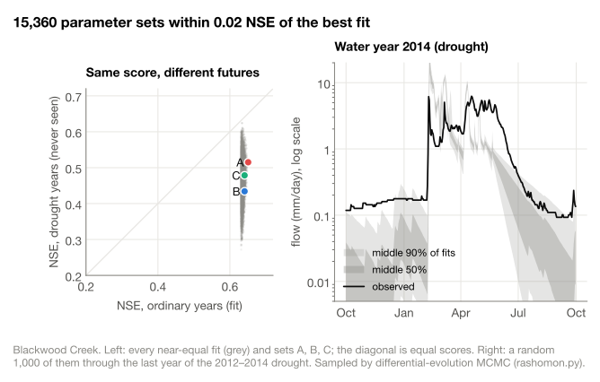
On the training years, the 15,360 fits span 0.02 NSE. On the droughts they span 0.27 to 0.62. Their median late-summer flow in ordinary years ranges from 1% to 158% of observed (5th–95th percentile). Within the set, a better training score barely predicts a better drought score (Spearman \(\rho = 0.10\)). This is underspecification in a creek. The metric you optimized can't choose between models that disagree about the case you care about.

The right panel is worse. In 2014 the whole ensemble fails the same way: winter baseflow too low, too much melt in a February warm spell, too little in spring. All but one of the 15,360 fits underpredict drought runoff, and the middle 90% deliver 60–83% of the observed volume. Averaging an ensemble of one architecture removes variance but keeps the shared bias.

The weights aren't physical constants

The parameter names invite you to read them as properties of the watershed. They behave like weights.

They move with the training distribution. Calibrated on the drought years, the melt threshold rises from 1.1 °C to 2.3 °C, \(\beta\) falls from 4.5 to 1.0, and soil capacity jumps to its 500 mm ceiling. The watershed didn't change. The data did.

They absorb errors in the inputs. In 1983 and 1984 the gauge recorded as much water as the gridded precipitation says fell. Forests evaporate hundreds of millimetres a year, so the precipitation input is probably too low. Gridded products built from mostly low-elevation gauges can miss much of the mountain precipitation in some Sierra storms.[] The model can't make water, so the evaporation parameter \(\text{LP}\) sits pinned at the bound that minimizes evaporation, in every fold. Even so, the best fit delivers only 74% of observed runoff. A “physical” parameter is compensating for a biased input, just as a network learns to correct a miscalibrated feature.

The priors can be wrong. The standard HBV-light ranges cap the leak from the fast to the slow store at 3 mm/day, and every calibration hits the cap. Removing it (the fit settles near 16 mm/day) raises NSE from 0.65 to 0.69 on the training years and from 0.52 to 0.57 on the droughts. Parameter bounds are a prior, and a prior is a hyperparameter. Fowler et al. found something similar for Australia's Millennium Drought. Many apparent failures of conceptual models there came from how they were calibrated, not from their structure.[]

The loss function picks the model. Fit on NSE of log flow, which weights a 0.1 mm/day trickle like a 10 mm/day flood, the same model scores worse on ordinary years (0.47) but better on droughts (0.63 vs 0.52).

Learning from more data: where “slower” is true and where it isn't

If calibration is training, it has a learning curve. Here the physics model faces a small transformer (two layers, \(d_{\text{model}} = 64\), a 365-day window of the same three inputs). Both maximize NSE on 5, 10 or 20 years with the same cross-validation folds, and neither ever trains on the droughts.

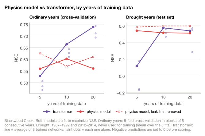
With 5 years of data, the physics model wins. It is slightly ahead on ordinary years and far ahead on droughts (0.54 vs 0.17 NSE). With 10 and 20 years the transformer pulls ahead on ordinary years (0.68 and 0.72) and catches up on droughts (0.56 and 0.59).[] The physics model doesn't improve: 0.56 held-out with 5 years, 0.56 with 20, peaking at 10. With 5 years it scores 0.78 on its training years and 0.56 on held-out ones. That's a classic overfit, from only eight parameters.

The transformer isn't a clean win. Its median late-summer flow is zero: it predicts negative flows in August and September, which are clipped to 0 before scoring. Its held-out NSE on log flow is −0.51, against the physics model's 0.37. Trained on the same flood-weighted loss, it fails where sets A and B fail, only worse, because nothing in its architecture says flow can't be negative. Buckets can't go negative, and that kind of constraint is worth writing by hand. (An LSTM with the same data scored about zero on the droughts. Single-basin networks are fragile.)

This is the bias–variance picture. A strong inductive bias is valuable when data are scarce and becomes a ceiling when they aren't, because the remaining error comes from structure, not parameters. It's Sutton's “bitter lesson”: general methods that scale with data and computation eventually beat encoded human knowledge.[] Hydrology learned it around 2019. A single LSTM trained on 531 CAMELS basins beat conceptual models calibrated basin by basin on a held-out decade.[] Nearing et al. argue that the theory in conceptual models acts as regularization and is what limits their generality.[] And my transformer is handicapped: it sees one basin, and networks trained on many basins do much better.[] The curve above understates learned models.

Now the pushback. “Slower” is false in wall-clock terms. On this Mac, a physics calibration took about 10 seconds on one CPU core. An LSTM took 10–30 seconds and the transformer 45–165 seconds per fit on the GPU, times three seeds. The physics model is slower in three other senses:

1. Slower to improve with data. The flat red line is the main result.
2. Slower to improve at all. Every gain needs a human to notice a residual and write a module, and some modules make things worse.
3. Slower to scale. Gradient-free search needed about 16,000 runs for 8 parameters, and it gets much worse as parameters are added. So the field is moving to differentiable conceptual models: the same buckets written in an autodiff framework and trained by gradient descent, often with a neural network predicting their parameters.[][] Trained across hundreds of basins, such models approach LSTM accuracy.[] At that point “physics or ML?” has no content left. It's a neural network with some layers written by hand.

On droughts the physics model's advantage is narrower than it looks. At 5 years it wins easily. At 20 years the two are close, and the best performer is the physics model with its prior removed. Its drought skill also depends heavily on which near-equal fit you happened to pick.

What to take from this

If a calibrated conceptual model is an ML model, hold it to ML standards. Hydrology reached several of them early:

• Report held-out scores, not calibration scores. Held-out blocks lose 0.09 NSE here, and the driest block loses 0.27.
• Test under shift on purpose, with Klemeš's differential split-sample test.
• Report the Rashomon set, not the argmin. Beven's GLUE did this in 1992.[] For anything the loss doesn't score (low flows, drought volumes, warming), the spread across near-equal fits is the uncertainty.
• Don't read the weights as physics. A parameter that hits its bound, drifts with the training period, or compensates for an input bias is a fitted weight with a physical name.
• Choose the loss for the decision. NSE is a flood score. If you care about August, train on August.

The physical structure buys something real. It suggests which module is missing, it conserves mass and forbids negative flow, and it works from five years of data. It doesn't exempt the model from the ways fitted models fail. On Blackwood Creek, the physics model and the transformer are both function approximators fit to one gauge. The difference is that nobody expects the transformer's weights to mean anything.

Code: the model, calibration, cross-validation, Hessian, and learning-curve scripts are in code-and-figures/. The Rashomon-set analysis and figure are rashomon.py and rashomon_figure.py. Data are CAMELS basin 10336660, downloaded by download.py.

Notes and References

1. USGS gauge 10336660, "Blackwood C nr Tahoe City CA," drainage area 11.2 mi² (29 km²), daily discharge since 1 October 1960. https://waterdata.usgs.gov/monitoring-location/10336660/. Roberts et al. (2018) describe its discharge as "strongly snowmelt-driven… typically peaking at over 300% of the annual mean in May or June": D. C. Roberts et al., "Snowmelt timing as a determinant of lake inflow mixing," Water Resources Research 54 (2018), doi:10.1002/2017WR021977. ^
2. A. J. Newman et al., "Development of a large-sample watershed-scale hydrometeorological data set for the contiguous USA," HESS 19 (2015): 209–223, doi:10.5194/hess-19-209-2015. This is 671 basins with daily forcing and USGS streamflow. I use its Daymet basin-average forcing. The name CAMELS comes from N. Addor et al., "The CAMELS data set: catchment attributes and meteorology for large-sample studies," HESS 21 (2017): 5293–5313, doi:10.5194/hess-21-5293-2017. Potential evaporation here is computed from temperature with the Hargreaves formula. ^
3. HBV was developed at the Swedish Meteorological and Hydrological Institute in the early 1970s: S. Bergström, The HBV model – its structure and applications, SMHI Reports Hydrology RH 4 (1992). The model here is a simplified HBV (no routing routine, no snow refreezing or liquid-water holding). Its parameter ranges come from J. Seibert and M. J. P. Vis, "Teaching hydrological modeling with a user-friendly catchment-runoff-model software package," HESS 16 (2012): 3315–3325, doi:10.5194/hess-16-3315-2012. ^
4. J. E. Nash and J. V. Sutcliffe, "River flow forecasting through conceptual models part I — A discussion of principles," Journal of Hydrology 10 (1970): 282–290, doi:10.1016/0022-1694(70)90255-6. \(\text{NSE} = 1 - \sum(\text{sim} - \text{obs})^2 / \sum(\text{obs} - \text{mean obs})^2\). A recent history argues its dominance "appears to be derived more from tradition than from any demonstration of technical superiority": L. A. Melsen et al., "The rise of the Nash-Sutcliffe efficiency in hydrology," Hydrological Sciences Journal 70 (2025), doi:10.1080/02626667.2025.2475105. ^
5. F. Kratzert et al., "Rainfall–runoff modelling using Long Short-Term Memory (LSTM) networks," HESS 22 (2018): 6005–6022, doi:10.5194/hess-22-6005-2018. The comparison there is visual: "albeit the LSTM was only trained to predict runoff from meteorological observations, it has learned to model snow dynamics without any forcing to do so." ^
6. T. Lees et al., "Hydrological concept formation inside long short-term memory (LSTM) networks," HESS 26 (2022): 3079–3101, doi:10.5194/hess-26-3079-2022. They used linear probes on 669 British basins, with ERA5-Land reanalysis as the target. ^
7. V. Klemeš, "Operational testing of hydrological simulation models," Hydrological Sciences Journal 31 (1986): 13–24, doi:10.1080/02626668609491024. ^
8. L. Coron et al., "Crash testing hydrological models in contrasted climate conditions: An experiment on 216 Australian catchments," Water Resources Research 48 (2012): W05552, doi:10.1029/2011WR011721. ^
9. K. Beven, "A manifesto for the equifinality thesis," Journal of Hydrology 320 (2006): 18–36, doi:10.1016/j.jhydrol.2005.07.007. ^
10. L. Breiman, "Statistical modeling: The two cultures," Statistical Science 16 (2001): 199–231, §8, doi:10.1214/ss/1009213726. ^
11. A. D'Amour et al., "Underspecification presents challenges for credibility in modern machine learning," JMLR 23 (2022): 1–61, https://jmlr.org/papers/v23/20-1335.html. ^
12. R. N. Gutenkunst et al., "Universally sloppy parameter sensitivities in systems biology models," PLoS Computational Biology 3 (2007): e189, doi:10.1371/journal.pcbi.0030189. This is 17 models whose eigenvalues "span many decades" and are "approximately evenly spaced in their logarithm." M. K. Transtrum et al., "Perspective: Sloppiness and emergent theories in physics, biology, and beyond," Journal of Chemical Physics 143 (2015): 010901, doi:10.1063/1.4923066. Here, the six unbounded parameters give eigenvalues of 43, 21, 1.9, 0.55, 0.17 and 0.012 (finite differences with 2% steps in rescaled coordinates, hessian.py). That spans 3.6 decades, with neighbours about 0.7 decades apart. The spectrum depends somewhat on the finite-difference step, because the model's thresholds make the loss slightly jagged. ^
13. H. V. Gupta et al., "Decomposition of the mean squared error and NSE performance criteria: Implications for improving hydrological modelling," Journal of Hydrology 377 (2009): 80–91, doi:10.1016/j.jhydrol.2009.08.003. ^
14. C. J. F. ter Braak, "A Markov Chain Monte Carlo version of the genetic algorithm Differential Evolution," Statistics and Computing 16 (2006): 239–249, doi:10.1007/s11222-006-8769-1. I ran 256 chains for 3,000 generations, all starting at the best fit, with a target that is uniform over the region scoring within 0.02 NSE of it. I kept every 25th generation of the second half. See rashomon.py. ^
15. D. Griffin and K. J. Anchukaitis, "How unusual is the 2012–2014 California drought?," Geophysical Research Letters 41 (2014): 9017–9023, doi:10.1002/2014GL062433. Precipitation was low but not unprecedented. Record heat made the moisture deficit extreme. ^
16. J. D. Lundquist et al., "High-elevation precipitation patterns: Using snow measurements to assess daily gridded datasets across the Sierra Nevada, California," Journal of Hydrometeorology 16 (2015): 1773–1792, doi:10.1175/JHM-D-15-0019.1. They found median water-year errors within ±10%, but individual storm errors sometimes exceeded 50%, which can bias a year by about 20%. They did not test Daymet, the product used here, so this is a plausible explanation, not a demonstrated one. Snow and groundwater carried across 1 October may also contribute. ^
17. K. J. A. Fowler et al., "Simulating runoff under changing climatic conditions: Revisiting an apparent deficiency of conceptual rainfall-runoff models," Water Resources Research 52 (2016): 1820–1846, doi:10.1002/2015WR018068. The standard test "often missed potentially promising parameter sets within a given model structure, giving a false negative impression of the capabilities of the model." For the opposite result, where conceptual models consistently overestimated runoff after drought shifted catchment behaviour, see M. Saft et al., "Bias in streamflow projections due to climate-induced shifts in catchment response," Geophysical Research Letters 43 (2016): 1574–1581, doi:10.1002/2015GL067326. ^
18. Numbers are 3-seed ensemble averages from my rerun of learning_curve.py, pooled over the five held-out blocks. Drought scores are the mean over the five fits. GPU training isn't bit-reproducible, so the figure (an earlier run of the same script) differs by up to about 0.05, but the ordering is the same. The physics numbers reproduce exactly. ^
19. R. Sutton, "The Bitter Lesson" (2019), http://www.incompleteideas.net/IncIdeas/BitterLesson.html. ^
20. F. Kratzert et al., "Towards learning universal, regional, and local hydrological behaviors via machine learning applied to large-sample datasets," HESS 23 (2019): 5089–5110, doi:10.5194/hess-23-5089-2019. The benchmarks included SAC-SMA, VIC, HBV, mHM and FUSE. ^
21. G. S. Nearing et al., "What role does hydrological science play in the age of machine learning?," Water Resources Research 57 (2021): e2020WR028091, doi:10.1029/2020WR028091. In their words, "it is the regularization in the traditional models (i.e., the hydrological theory…) that is actually the cause of their lack of generality." ^
22. F. Kratzert et al., "HESS Opinions: Never train a Long Short-Term Memory (LSTM) network on a single basin," HESS 28 (2024): 4187–4201, doi:10.5194/hess-28-4187-2024. ^
23. C. Shen et al., "Differentiable modelling to unify machine learning and physical models for geosciences," Nature Reviews Earth & Environment 4 (2023): 552–567, doi:10.1038/s43017-023-00450-9. ^
24. W.-P. Tsai et al., "From calibration to parameter learning: Harnessing the scaling effects of big data in geoscientific modeling," Nature Communications 12 (2021): 5988, doi:10.1038/s41467-021-26107-z. They call traditional calibration "highly inefficient," producing "non-unique solutions." Their large speed-ups are for a land-surface model (VIC), not HBV. ^
25. D. Feng et al., "Differentiable, learnable, regionalized process-based models with multiphysical outputs can approach state-of-the-art hydrologic prediction accuracy," Water Resources Research 58 (2022): e2022WR032404, doi:10.1029/2022WR032404. This is a median NSE of 0.732 over 671 CAMELS basins, against 0.748 for an LSTM. Their HBV has neural networks embedded in some modules. ^
26. K. Beven and A. Binley, "The future of distributed models: model calibration and uncertainty prediction," Hydrological Processes 6 (1992): 279–298, doi:10.1002/hyp.3360060305. This paper introduced GLUE. ^