Machine Learning in Slow Motion
Building a physics model with fitted parameters is machine learning, but slower
September 2026
Physics models are sometimes thought of as a cleaner alternative to machine learning: you get interpretable parameters and less overfitting. But when you have unknown parameters in a model, you have to fit them to data. That starts to look a lot like machine learning, only with a human slowly defining the rules and parameters instead of an algorithm.
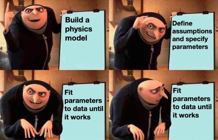
In some cases, the choice of whether to use a physics model or a machine learning model is obvious. If you're modeling planets with Newton's laws, go for physics. If your goal is protein folding, physics is way too expensive and ML is the clear pick.
The ambiguous cases happen when:
- The physical laws are known, but not perfectly
- Your model depends on constants that are measured or assumed, rather than fundamental physical constants alone
- You have a medium amount of data: not so little that machine learning is useless, and not so much that it's excellent
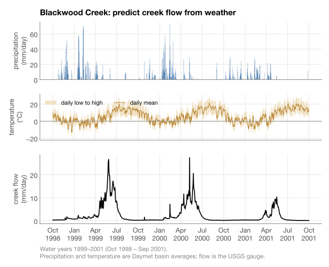
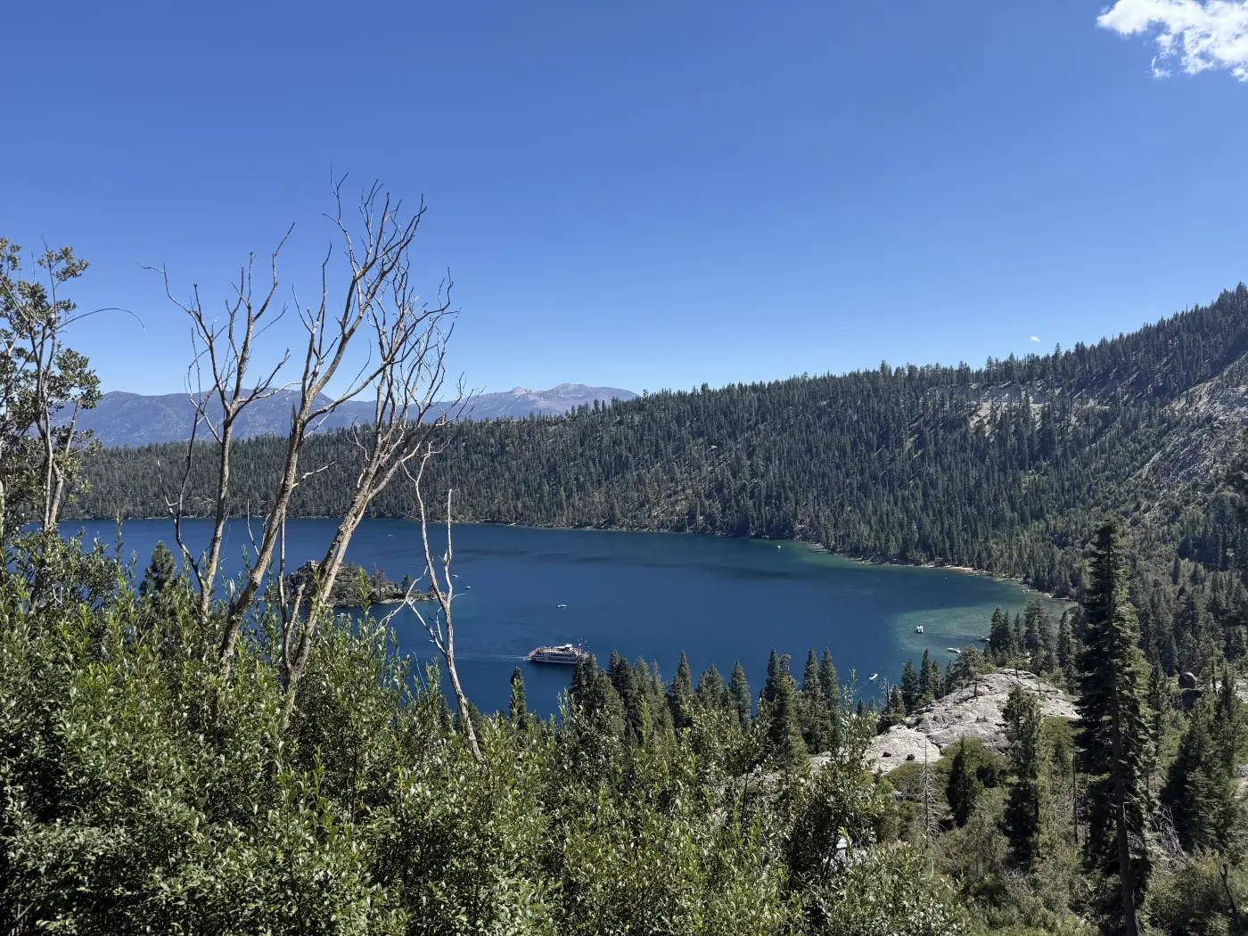
One such example is predicting the flow of water in a creek given the time series of precipitation and temperature. We're going to do this with data for Blackwood Creek, near Lake Tahoe in California, and we'll see how the physics model measures up against a bitter lesson transformer, and how interpretable its parameters really are.
The silly solution is: however much it flows on average, just guess that number. To make sure this isn't what's happening, the metric we'll use is NSE, which looks at the error we would get if we used the “predict the same as the average” strategy and computes how much of that we eliminated. 0 means we are no better than the silly strategy; 1.0 means we are perfect; a negative means we are actively worse than just guessing the average.[]
NSE formula
\[ \text{NSE} = 1 - \frac{\sum_t \left( Q_{\text{sim}}(t) - Q_{\text{obs}}(t) \right)^2}{\sum_t \left( Q_{\text{obs}}(t) - \bar{Q}_{\text{obs}} \right)^2} \]
where \(Q_{\text{obs}}(t)\) is the observed flow on day \(t\), \(Q_{\text{sim}}(t)\) is the model's prediction, and \(\bar{Q}_{\text{obs}}\) is the average observed flow. The fraction is the model's squared error divided by the squared error of always guessing the average. Because the errors are squared, days with high flow count much more than days with low flow.
Building the Model
To model the data, we'll use a simplified version of a standard model in hydrology.[][] You'll notice we keep adding new parameters and rules to improve the fit.
Let's start with the simplest possible model: a leaky bucket of water. When it rains, all that water collects in the bucket. Every day, a fraction \(k\) drains from the bucket — that's our flow. Let's simulate this, and fit the \(k\) that best models our data.
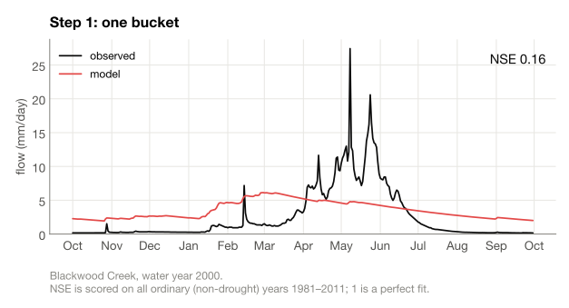
As you can see from the chart, this model is far too simple. This is the point where a modeler typically adds more rules and parameters in order to better model the data.
Next, we are going to add snow and melting. If today's temperature \(T(t)\) is below a certain temperature \(T_{\text{melt}}\) then instead of rain going into the bucket, we get snow that piles up. When it gets above \(T_{\text{melt}}\), the snow melts at a rate \(M(t)\) in mm/day, set by a melt factor \(f_{\text{melt}}\):
\[ M(t) = f_{\text{melt}} \cdot \left(T(t) - T_{\text{melt}} \right). \]
The warmer it is, the faster the snow melts. When we add snow accumulation and melting to our model according to this rule, the results are much better.
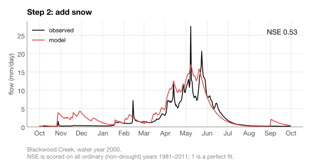
The cost is that now we have two new parameters to fit: \(f_{\text{melt}}\), the melting rate constant, and \(T_{\text{melt}}\), the daily mean temperature required for melting.
Until this point we had one leaky bucket with rate \(k\). Now let's try two leaky buckets: one fast-draining, and one slow-draining. Whatever drains out of these is the flow for the creek. We'll also add a third bucket, for the soil at the top.
- Soil: when it rains or the snow melts, some of that water soaks into the soil. New parameter: soil capacity.
- Runoff: some rain and snowmelt goes to the fast bucket instead of the soil. New parameter runoff curve shape \(\beta\) sets the shape of the curve based on how full the soil is.
- Fast and slow buckets: two new parameters for their drain rates.
- Leak: some water leaks from the fast bucket to the slow one. New parameter: leak rate.
- Evaporation: the soil loses water to evaporation and plants. Less if it's dry, more if it's wet, up to a maximum rate based on an estimate from prior research.[] New parameter: evaporation threshold where we hit the maximum rate.
Splitting the buckets is only a modeling choice: it doesn't tell us about real sections of the groundwater and their drainage times.
Soil and evaporation equations
If \(I(t)\) is the rain plus snowmelt on day \(t\) and \(S_{\text{soil}}(t)\) is the water in the soil, the amount \(F(t)\) that goes to the fast bucket is \[ F(t) = I(t) \cdot \left( \frac{S_{\text{soil}}(t)}{C_{\text{max soil}}} \right)^{\beta}, \] and the remaining \(I(t) - F(t)\) stays in the soil. \(C_{\text{max soil}}\) here is the soil's maximum water capacity. Evaporation and plant use take \[ E(t) = E_{\text{pot}}(t) \cdot \min\left( \frac{S_{\text{soil}}(t)}{f_{\text{LP}} \cdot C_{\text{max soil}}}, 1 \right) \] out of the soil each day, where \(E_{\text{pot}}(t)\) is the maximum evaporation rate. The evaporation threshold can't be more than the soil capacity, so it's written as a fraction \(f_{\text{LP}}\) of it, and \(f_{\text{LP}}\) is the fitted parameter.
The maximum rate \(E_{\text{pot}}\) is given by Hargreaves as \[ E_{\text{pot}}(t) = 0.0023 \cdot R_a(t) \cdot \left( T(t) + 17.8 \right) \cdot \sqrt{T_{\text{max}}(t) - T_{\text{min}}(t) } \] where \(R_a(t)\) is the sunlight energy at the top of the atmosphere at that latitude and time of year, expressed as mm/day of water it could evaporate; \(T(t)\) is the mean temperature that day; \(T_{\text{max}}\) is the high temperature that day; and \(T_{\text{min}}\) is the low temperature that day.
0.0023 and 17.8 aren't fundamental physical constants. 0.0023 combines a coefficient fit to eight years of grass measurements in Davis, California[] with a second fitted coefficient for estimating sunlight from temperature. 17.8 comes from converting the original Fahrenheit equation to Celsius.[]
Now that we added another six parameters, for eight total, is our fit any better?
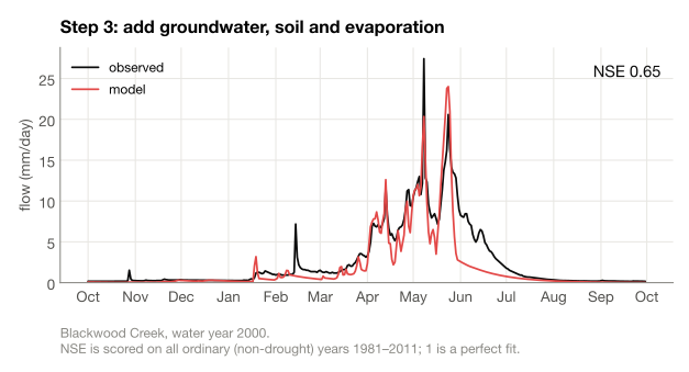
There's a noticeable improvement in the fit, especially around the fall and winter.
Choosing Parameters is Machine Learning
I used a technique called differential evolution[] in order to optimize this model. Although we have just 8 parameters instead of billions or trillions like in an LLM, using differential evolution to fit those eight parameters is machine learning.
Here we were able to do machine learning to find good parameters because each simulation takes milliseconds. In climate modeling, for example, each simulation takes so much time that exploring the full parameter space by algorithm is often too expensive, so you have to use slow-motion manual tuning. Tuning parameters is a difficult art and science, requiring expert judgment.[]
Fake Interpretability
You might think that having parameters with a clear physical meaning, like the snow melting temperature, improves the interpretability of the model. But this is often an illusion: parameter values can easily bend to compensate for missing structure in your model.[]
In our model, we constrained the leak rate to a standard range of 0-3 mm/day.[] But all the fits I found above 0.64 NSE pushed it all the way to 3 mm/day. If we remove the constraint, it jumps all the way up to 16 mm/day!
Removing that constraint doesn't overfit: it turned out to improve model performance on drought years, and on held-out years with 20 years of training data. It also shifted values for a lot of the other parameters like soil capacity.
This doesn't mean the real leak rate is that high, or that the new soil capacity is correct. The “leak rate” in our model is really just a parameter that does some math, not a claim on a real-world physical effect. Increasing this parameter happens to model the data better.
Since this kind of compensation is very possible even in a physically motivated model, it can be dangerous to assume the parameters that pop out of your model are “interpretable”. They could be doing math to model very different physical phenomena than what they're meant to represent.
Some Parameter Changes are Invisible
When we fit to the data, we end up with some parameters. But there might be another set of parameters that scores about the same, but has some very different values. We can't tell from the data and the physical model alone whether the parameters match the real-world quantities they're meant to represent.
I picked out some examples that are within 0.01 NSE of the best fit, but have very different parameters.
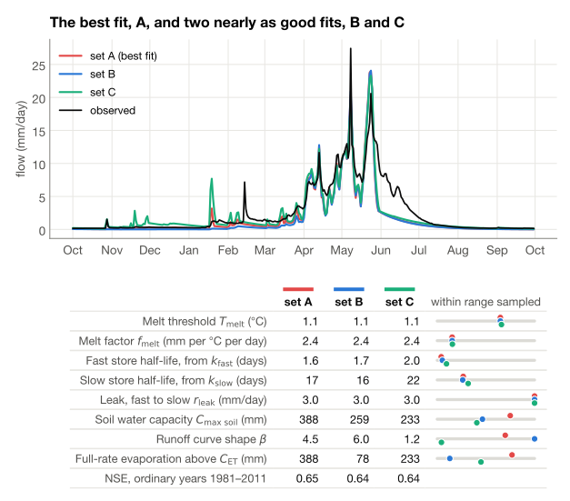
While these parameter changes don't really affect the NSE score, that doesn't mean they don't matter. The three models behave very differently on the late summer subset of the dataset.
Models A and B are up to 8-11x below observed flow values in the late summer, while C is pretty close. This is almost invisible on the full chart because late summer flow is so small compared to the rest of the year.
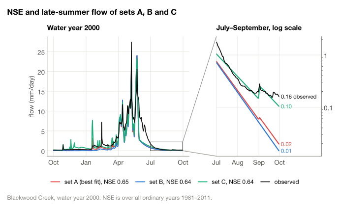
Even though model A is up to 8x too low on these months of 2000, it's the best fit. That's because we're optimizing for NSE, which barely cares about data with small absolute values.
Finding Parameter Trade-offs
Once you have your model, how can you tell which parameters aren't very meaningful for the score?
Often, it's not that one parameter is totally useless, but that multiple parameter changes cancel out in a way that leaves the score about the same. There's a mathematical tool that can quantify these trade-offs: the Hessian, which is kind of a multivariable second derivative.
Its eigenvectors are directions in parameter space, and each one's eigenvalue says how fast the score changes as you move that way: a large eigenvalue means the fit pins that direction down, a small one means it can drift without doing much.
The math
We start with our loss \(L\) as function of our parameters, \(\theta\). In this case, \(L(\theta) = -\text{NSE}(\theta) \). What we want to do is find: if we change our parameters by some vector \(\Delta\), how much does the loss change? It would be especially interesting to know which parameter changes have the biggest impact and which have the smallest impact.
Now we define the Hessian. This is a square matrix, where the entries are partial derivatives like
\[ H_{ij} = \frac{\partial^2 L}{\partial \theta_i \, \partial \theta_j}. \]
So if we fill that out for parameters \(\theta_1,\dots,\theta_n\), we get a matrix like
\[ H = \begin{pmatrix} \frac{\partial^2 L}{\partial \theta_1^2} & \frac{\partial^2 L}{\partial \theta_1 \partial \theta_2} & \cdots & \frac{\partial^2 L}{\partial \theta_1 \partial \theta_n} \\ \frac{\partial^2 L}{\partial \theta_2 \partial \theta_1} & \frac{\partial^2 L}{\partial \theta_2^2} & \cdots & \frac{\partial^2 L}{\partial \theta_2 \partial \theta_n} \\ \vdots & \vdots & \ddots & \vdots \\ \frac{\partial^2 L}{\partial \theta_n \partial \theta_1} & \frac{\partial^2 L}{\partial \theta_n \partial \theta_2} & \cdots & \frac{\partial^2 L}{\partial \theta_n^2} \end{pmatrix}. \]
Notice that \(H\) is symmetric: \(H = H^\top\). By the spectral theorem, this means it has real eigenvalues and orthogonal eigenvectors.
Let's use our best fit model as a reference. Since it's the best fit, it's a local minimum for loss, so the loss surface looks like a bowl nearby. It turns out that if we move a distance \(s\) along an eigenvector of this matrix, we can predict the change in loss from its eigenvalue \(\lambda_k\) using Taylor expansion:
\[ \Delta L \approx \tfrac{1}{2} \lambda_k s^2. \]
If we want to find how far we can go in a direction before the loss changes by some small amount, we can solve for \(s_k\).
This tells us something important: once we have the eigenvectors of the Hessian, we know which directions in parameter space the model pins down the most, and which can move around without doing much. A direction that matters a lot for the fit is called “stiff”, while one that's more flexible without changing much is called “sloppy”.[]
In our case, our stiffest eigenvector has \(\lambda_1=43.4\). It's 66% along the melt threshold direction and 34% along melt factor, indicating that these two parameters are similar for all the nearby best fits. We can only adjust the parameters by 2% of their range in this direction before our loss goes up by 0.01.
Meanwhile, the sloppiest eigenvector has \(\lambda_6=0.0115\). This is 91% along the runoff curve shape \(\beta\) direction and 9% along the soil capacity direction, indicating that choosing different values for these two parameters is less impactful for the loss. We can move parameters across the entire range in this direction and barely touch the loss.
And indeed, if we look at the difference between models A and C (both good fit models with very different parameters), the line between them is only 11° off from our sloppiest direction.
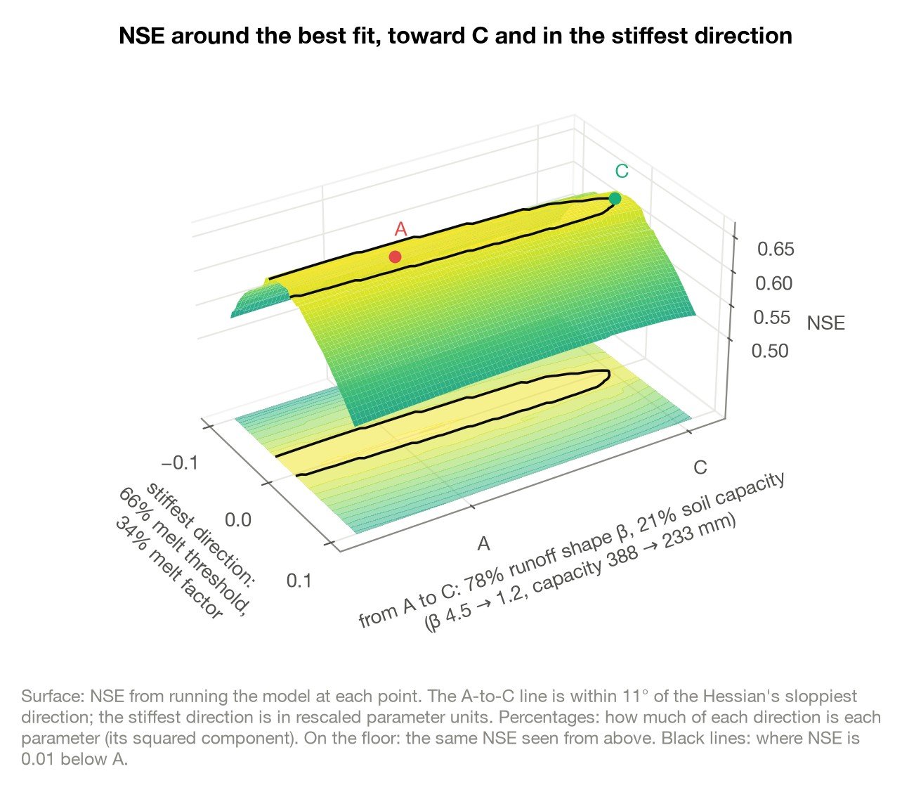
This means that once we have a best fit, it's cheap to use the Hessian eigenvectors to figure out which parameters are vital to a good fit, and which are more loose.
Physics vs ML
Some common claimed advantages for physics models over ML models are:
- Better interpretability
- Better generalization outside the training data
We saw that the interpretability of a physics model can sometimes be fake, since very different parameter choices can lead to similar accuracy. To see if the generalization claim holds up, I trained a transformer on the same dataset. No three buckets, no leak rate. Just a bitter-lesson-pilled transformer with 67,265 parameters. I trained three independent models and used their ensemble as the ML predictor.
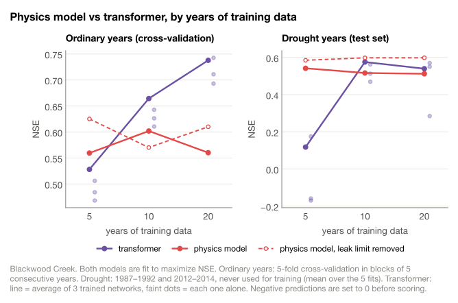
With only five years of data, the physics models won on both tests, most clearly on drought years (0.54–0.59 NSE against 0.12 for the transformer). By 10 years the transformer had caught up: it beat both physics models on ordinary years and the standard one on drought years. However, even with 20 years of data, the best drought model overall was the physics model with the leak limit removed.
So how do we choose between physics models and less constrained ML?
If you're working with established physics and no parameters to fit, like Newton's laws, physics is definitely the better choice. You know it works and don't need a dataset.
Sometimes you need a dataset even for established laws, like Ohm's law \(V=IR\) when you don't know the resistance \(R\). Simple linear fits like these are usually helpful, interpretable, and useful for understanding the physics.
In other cases, where you're fitting quite a few parameters and making a lot of assumptions about the underlying physical model, machine learning can be the right choice even if you've found some equations that approximate the system.[] Here, it matched or beat the physics model on ordinary years once it had enough data, though a physics model still did best on drought years. And the physical interpretability of a model might be questionable anyway.
This doesn't apply only to physics either. You can run into the same issues anywhere you're fitting parameters to a mathematical model of something in the real world, like ecology, epidemiology, or some models of biology. If your model has a lot of fitted and unknown parameters, it's worthwhile to treat it as a machine learning model, because that's what it is. This means testing on held out data and edge cases, and comparing to other models of the data even if your initial model works well.
The process of defining assumptions, setting parameters, and measuring results has a lot more in common with machine learning than it seems. In fact, if you automate the parameter search instead of hand-tuning, it is machine learning. So before building a physically motivated model, it's worth checking if it really helps you understand the underlying system, or if you have enough data that you'd get a better result faster by just throwing some machine learning at it.
References
The GitHub for this project is at crackalamoo/blog-demos.
- Development of a large-sample watershed-scale hydrometeorological data set for the contiguous USA: data set characteristics and assessment of regional variability in hydrologic model performance (A. J. Newman et al., Hydrology and Earth System Sciences, 2015) ^
- Nash–Sutcliffe model efficiency coefficient (Wikipedia) ^
- Development and application of a conceptual runoff model for Scandinavian catchments (Sten Bergström, SMHI, 1976) ^
- Teaching hydrological modeling with a user-friendly catchment-runoff-model software package (Jan Seibert & Marc Vis, Hydrology and Earth System Sciences, 2012) ^
- Crop evapotranspiration: Guidelines for computing crop water requirements (FAO Irrigation and Drainage Paper 56) (Richard G. Allen, Luis S. Pereira, Dirk Raes & Martin Smith, FAO, 1998) ^
- Hargreaves Method (HEC-HMS Technical Reference Manual, US Army Corps of Engineers) ^
- Evapotranspiration (HEC-HMS User's Manual 4.8, US Army Corps of Engineers) ^
- Differential Evolution – A Simple and Efficient Heuristic for Global Optimization over Continuous Spaces (Rainer Storn & Kenneth Price, Journal of Global Optimization, 1997) ^
- The Art and Science of Climate Model Tuning (Frédéric Hourdin et al., Bulletin of the American Meteorological Society, 2017) ^
- Universally Sloppy Parameter Sensitivities in Systems Biology Models (Ryan N. Gutenkunst et al., PLOS Computational Biology, 2007) ^
- Towards learning universal, regional, and local hydrological behaviors via machine learning applied to large-sample datasets (Frederik Kratzert et al., Hydrology and Earth System Sciences, 2019) ^
- To bucket or not to bucket? Analyzing the performance and interpretability of hybrid hydrological models with dynamic parameterization (Eduardo Acuña Espinoza et al., Hydrology and Earth System Sciences, 2024) ^
Footnotes
- We don't necessarily want 0 °C for \(T_{\text{melt}}\) because it represents a daily mean air temperature at which snow melts: we aren't physically measuring the temperature of the snow, and don't account for day-night swing, so we need a fitted parameter. ^
- Two of our parameters, the leak rate and the evaporation threshold, were at the edge of their ranges and so were not at local minima. We kept them constant and ran the Hessian analysis with the other six parameters.^